Basic Run¶

A single parcel simulation from initial conditions through droplet activation, using a two-mode aerosol population (accumulation + Aitken). Demonstrates the core API: constructing an aerosol population, running the model, and accessing the trajectory and activation diagnostics.

Script: examples/basic_run.py

python examples/basic_run.py
python examples/basic_run.py --V 0.5 --T0 283.0 --t-end 200.0 \
    --out output/run.nc --plot output/run.png

Setup¶

import pyrcel as pm

accumulation = pm.AerosolSpecies(
    "accumulation",
    pm.Lognorm(mu=0.05, sigma=2.0, N=1000.0),  # mu in µm
    kappa=0.54,
    bins=50,
)
aitken = pm.AerosolSpecies(
    "aitken",
    pm.Lognorm(mu=0.01, sigma=1.6, N=2000.0),  # mu in µm
    kappa=0.3,
    bins=50,
)

model = pm.ParcelModel(
    [accumulation, aitken], V=1.0, T0=283.0, S0=-0.02, P0=85000.0, console=True
)
out = model.run(100.0, output_dt=1.0, terminate=False, progress=True)

The accumulation mode (\(\mu = 50\) nm, \(\sigma = 2.0\), \(\kappa = 0.54\)) represents sulfate-like particles that activate readily. The Aitken mode (\(\mu = 10\) nm, \(\sigma = 1.6\), \(\kappa = 0.3\)) is smaller and less hygroscopic; only a small fraction of Aitken bins exceed their critical supersaturation at this updraft speed.

Activation summary¶

pyrcel v2 — basic run
─────────────────────────────────────────────────────────────────
 Initial conditions
   T₀  =  283.15 K    P₀  =  85000 Pa    S₀  =  -0.0200
   V   =  1.00 m/s    accom = 1.00

 Aerosol population
   sulfate  N=1000.0 cm⁻³  μ=0.050 μm  σ=2.00  κ=0.54  bins=100

 Integration  t_end=300 s  output_dt=1 s  terminate=True  depth=10 m
─────────────────────────────────────────────────────────────────
 Activation summary
   S_max         =  0.4823 %
   t(S_max)      =  93.4 s
   z(S_max)      =  93.4 m
   N_act         =  6.23e+08 m⁻³
   act_frac      =  0.623

 Per-species
   sulfate  eq_act=0.621  nd_frac=0.623  Nd=6.23e+08 m⁻³
─────────────────────────────────────────────────────────────────
Wrote output/jax_basic_run.nc

Output figure¶

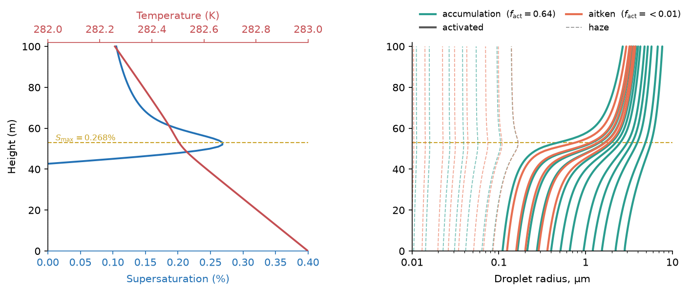
Parcel trajectory and aerosol size evolution

Left panel — supersaturation \(S\) (blue, bottom axis) and temperature \(T\) (red, top axis) as functions of height. The supersaturation rises as the parcel lifts, peaks at \(S_\text{max}\) (dashed gold line), then falls as condensation depletes water vapor faster than adiabatic cooling can generate it.

Right panel — size evolution of a sub-sample of aerosol bins from both modes (teal = accumulation, orange = Aitken). Bold solid traces are activated droplets (\(S_\text{crit} < S_\text{max}\)); dashed traces remain as haze. The kink in each activated trace marks the moment the droplet crosses its Köhler critical radius and begins growing freely.

Saving output¶

# NetCDF (CF-flavoured xarray dataset)
out.to_netcdf("run.nc")

# Pandas DataFrames (mirrors v1 tuple output)
parcel_df, aer_dfs = out.to_pandas()

# Parquet for fast downstream analysis
out.to_parquet("run.parquet")

See ModelOutput for the full list of format conversions.