Sensitivity Sweep: Exact vs Numerical ∂Smax/∂V

Compares the sensitivity of peak supersaturation \(\partial S_\text{max}/\partial V\) computed two ways — via the exact adjoint (jax.grad) and via numerical central-difference approximation — for each of three methods:

Method	Implementation	Exact gradient source
Parcel model	Full ODE (JAX/diffrax)	jax.grad through the integrator (adjoint)
ARG2000	Closed-form	jax.grad (analytical)
MBN2014	Iterative	jax.grad via implicit function theorem (IFT)

The figure has three columns per row: the exact adjoint, the numerical central-difference estimate on an extended grid, and the signed error (exact − numerical). Comparing the first two columns reveals where finite-difference approximation on a coarse grid diverges from the true gradient; the third column makes the discrepancy explicit and symmetric.

Script: examples/sensitivity_sweep.py

python examples/sensitivity_sweep.py              # compute, cache, plot
python examples/sensitivity_sweep.py --recompute  # force fresh sweep
python examples/sensitivity_sweep.py --no-plot    # cache only
python examples/sensitivity_sweep.py --cache PATH --plot PATH

Caching

The parcel model requires one JIT-compiled forward pass and one adjoint call per grid point (100 points on the default 10 × 10 grid). Results are saved to a compressed .npz cache so the figure can be regenerated without re-running the integrator:

import numpy as np

data = np.load("output/sensitivity_sweep_cache.npz")
smax_parcel            = data["smax_parcel"]            # shape (n_V, n_mu)
dsmax_dV_parcel_exact  = data["dsmax_dV_parcel_exact"]  # exact adjoint
dsmax_dV_parcel_num    = data["dsmax_dV_parcel_num"]    # numpy.gradient
V_grid                 = data["V_grid"]
mu_grid                = data["mu_grid"]

The cache is invalidated automatically if the grid dimensions or aerosol parameters differ between runs.

How adjoint and numerical gradients are computed

For the parameterizations, the exact gradient is a single jax.grad call:

import jax
import jax.numpy as jnp
from pyrcel.activation import arg2000

def smax_arg(V, mu):
    s, _, _ = arg2000(
        V, 283.0, 85000.0,
        jnp.array([mu]), jnp.array([2.0]),
        jnp.array([1000.0]), jnp.array([0.54]),
    )
    return s

dS_dV_exact = jax.grad(smax_arg, argnums=0)(1.0, 0.05)

For the parcel model, the adjoint is computed the same way but the function wraps the ODE integrator. The output time grid ts varies with V (to keep the integration horizon near ~1500 m for every grid point), so it is passed as an explicit argument alongside the other inputs so the JIT-compiled kernel is reused across the grid:

from pyrcel.integrator import max_supersaturation
from pyrcel.updraft import ConstantV

def smax_parcel(V_val, y0, r_drys, Nis, kappas_arr, ts):
    return max_supersaturation(
        y0, (r_drys, Nis, kappas_arr, accom, ConstantV(V_val)), ts
    )

grad_parcel = jax.jit(jax.grad(smax_parcel, argnums=0))
dS_dV_exact = grad_parcel(V_val, y0, r_drys, Nis, kappas_arr, ts)

The JIT compilation happens once on the first call; all subsequent grid points reuse the compiled kernel. Passing ts as an argument does not bias the gradient: by the envelope theorem, d(S_max)/d(t_end) = 0 whenever the supersaturation peak is strictly interior to [t0, t_end], so the ∂S_max/∂t_end · dt_end/dV coupling term vanishes identically.

Numerical gradient

The numerical approximation is computed on an extended grid — one extra log-spaced node in each direction beyond the original (V, μ) grid — so that every original node uses a central difference rather than a one-sided estimate. The gradient values are then interpolated back to the original grid using bilinear interpolation in log(V) × log(μ) space:

import numpy as np
from scipy.interpolate import RegularGridInterpolator

# Evaluate S_max on the extended grid, then take central differences.
dsmax_dV_ext = np.gradient(smax_ext, V_ext, axis=0)

# Interpolate back to original nodes in log-space.
interp = RegularGridInterpolator(
    (np.log10(V_ext), np.log10(mu_ext)),
    dsmax_dV_ext, method="linear",
)
coords = np.array([[np.log10(V), np.log10(mu)] for V in V_grid for mu in mu_grid])
dsmax_dV_num = interp(coords).reshape(len(V_grid), len(mu_grid))

Output figure

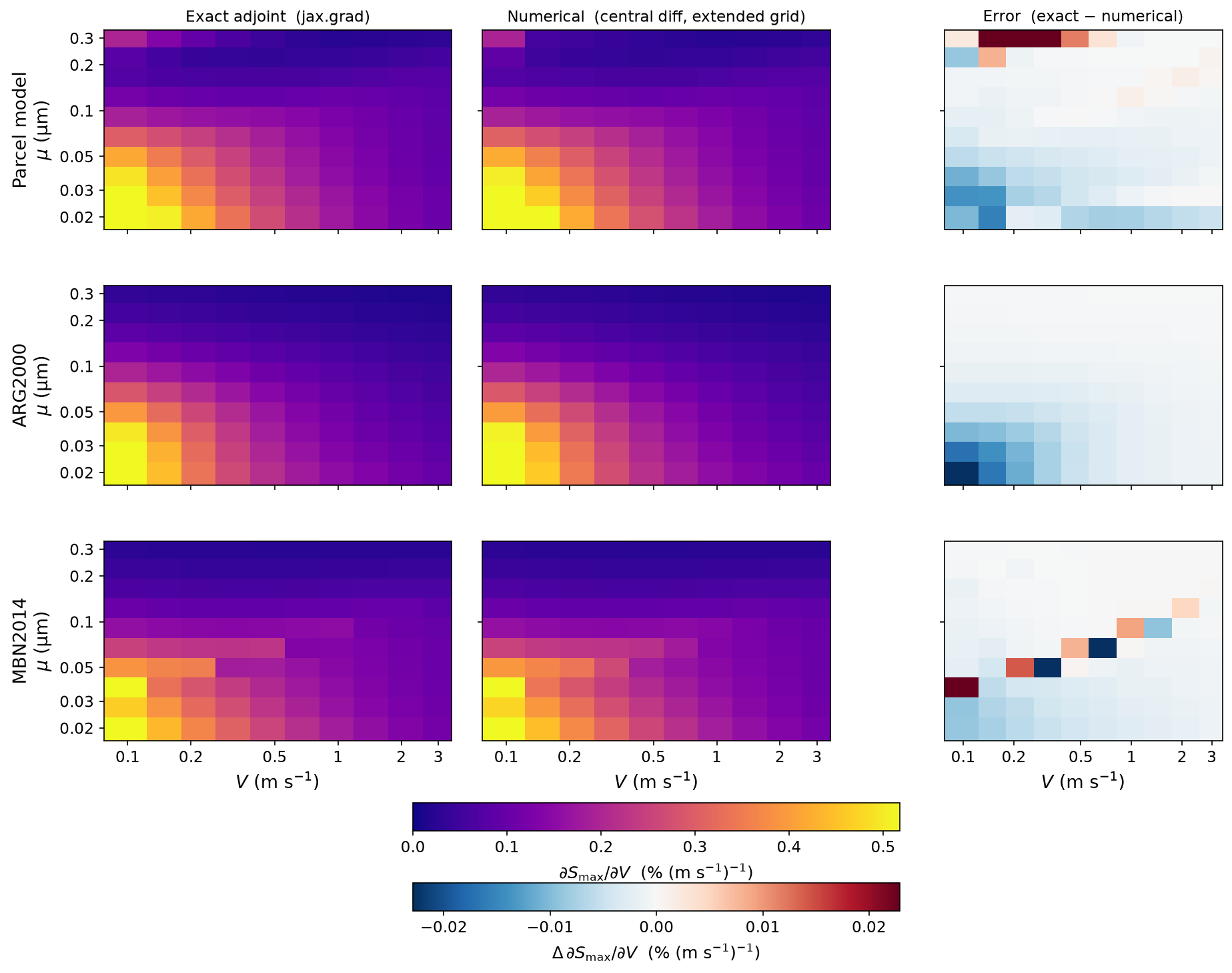
Layout: 3 rows × 3 columns. Each row is one method.

Column	Content	Colormap
Left	Exact adjoint (jax.grad)	plasma (0 → max)
Centre	Numerical (central diff, extended grid)	plasma, shared scale
Right	Signed error: exact − numerical	RdBu_r, symmetric about 0

Two horizontal colorbars are shown below the grid: one shared plasma scale for the left and centre columns, and one symmetric diverging scale for the error column. Both scales are global across all three rows.

Parcel model (row 1). The adjoint is obtained by backpropagating through the full ODE solver using a cubic Hermite interpolant constructed post-hoc from the saved discrete trajectory (SaveAt(ts=ts)). The ODE right-hand side supplies exact endpoint derivatives at the three bracket points, and the supersaturation peak is located analytically by solving the resulting quadratic dp/du = 0 — eliminating the aliasing that arises when the adaptive integrator's step structure shifts with V. The error column shows light blue across most of the domain (exact slightly < numerical), reflecting the O(h⁴) truncation error in the Hermite peak finder at the ~5 s output spacing, with warm tones at large μ where the S_max surface is very flat and the coarse extended-grid numerical estimate has poor signal-to-noise.

ARG2000 (row 2). The closed-form parameterization is fully differentiable at negligible cost. The error column is nearly white across most of the domain, confirming that the two methods agree closely and providing a sanity check for both the adjoint and the extended-grid numerical approach.

MBN2014 (row 3). Uses a jax.custom_vjp wrapper over a while_loop bisection, with the implicit function theorem (IFT) supplying the backward pass. Gradients are available across the full (V, μ) range, including the "critical" population-splitting regime (large μ) that previously produced NaN due to a sqrt(max(x, 0)) anti-pattern in the backward pass. The error column shows the largest signed residuals along the critical-branch boundary, where both the IFT gradient and the coarse-grid numerical estimate are least smooth.