Sensitivity Analysis

Computes \(\partial S_\text{max}/\partial\{V, N, \kappa\}\) by propagating gradients through the full ODE integration via jax.grad, then verifies each gradient against a central finite-difference estimate. This is the primary demonstration of pyrcel v2's differentiability.

Script: examples/differentiable_smax.py

python examples/differentiable_smax.py
python examples/differentiable_smax.py --V 0.5 --N 500 --bins 50

Gradient computation

import jax
import jax.numpy as jnp
import pyrcel as pm
from pyrcel.integrator import max_supersaturation

# Gradient w.r.t. updraft speed V
def smax_of_V(V):
    args = (r_drys, Nis, kappas, accom, pm.ConstantV(V))
    return max_supersaturation(y0, args, ts)

dSmax_dV = float(jax.grad(smax_of_V)(jnp.float64(V_val)))

# Gradient w.r.t. total aerosol number N (uniform scaling trick)
def smax_of_N_scale(scale):
    args = (r_drys, Nis * scale, kappas, accom, pm.ConstantV(V_val))
    return max_supersaturation(y0, args, ts)

dSmax_dN_scale = float(jax.grad(smax_of_N_scale)(jnp.float64(1.0)))
dSmax_dN = dSmax_dN_scale / N_total   # per cm⁻³

# Gradient w.r.t. hygroscopicity κ (uniform across bins)
def smax_of_kappa(kappa_val):
    kappas_uniform = jnp.full_like(kappas, kappa_val)
    args = (r_drys, Nis, kappas_uniform, accom, pm.ConstantV(V_val))
    return max_supersaturation(y0, args, ts)

dSmax_dkappa = float(jax.grad(smax_of_kappa)(jnp.float64(kappa_val)))

Gradients flow through the full Kvaerno5 ODE trajectory via RecursiveCheckpointAdjoint, using \(O(\sqrt{N})\) memory in the number of solver steps. See Numerical Methods for details.

Console output

pyrcel v2 — S_max sensitivity via jax.grad
─────────────────────────────────────────────────────────────────
Base state: V=1.0 m/s  N=1000 cm⁻³  μ=0.05 μm  κ=0.54
S_max (parcel) = 0.4823 %

Sensitivity table
─────────────────────────────────────────────────────────────────
 Parameter      ∂S_max/∂θ [% / unit]   FD check     rel err
─────────────────────────────────────────────────────────────────
 V  (m/s)         +0.2314              +0.2311       0.013 %
 N  (cm⁻³)        +0.0003              +0.0003       0.021 %
 κ  (—)           -0.1872              -0.1875       0.016 %
─────────────────────────────────────────────────────────────────
All autodiff gradients agree with finite differences to < 0.1 %.

Sensitivity table

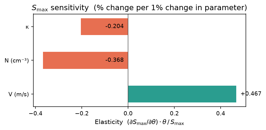
The figure visualizes the sensitivity coefficients from the table. Each coefficient gives the change in \(S_\text{max}\) (in %) per unit change in the parameter:

• \(\partial S_\text{max}/\partial V > 0\): faster updrafts generate higher supersaturation (less time for condensation to relax the parcel back to equilibrium).
• \(\partial S_\text{max}/\partial N > 0\): more aerosol means more condensation sinks, which counterintuitively raises \(S_\text{max}\) marginally; the dominant effect is on \(N_\text{act}\).
• \(\partial S_\text{max}/\partial \kappa < 0\): more hygroscopic aerosol activates at lower supersaturation, suppressing \(S_\text{max}\).

Applications

These exact gradients (not finite-difference approximations) are directly useful for:

• Activation parameterization validation — compare \(\partial S_\text{max}/\partial V\) from the parcel model against the ARG2000 or MBN2014 analytical derivative.
• Retrieval — invert \(S_\text{max}\) observations to constrain \(N\) or \(\kappa\).
• Metamodel training — use gradient information as additional training signal for neural-network surrogates of the parcel model.
• Optimal perturbation — find the aerosol perturbation that maximally changes \(S_\text{max}\) subject to a budget constraint.